Context

Computing accurate WCET on modern complex architectures is a challenging task. This problem has been devoted a lot of attention in the last decade but there are still some open issues. First, the control flow graph (CFG) of a binary program is needed to compute the WCET and this CFG is built using some internal knowledge of the compiler that generated the binary code; moreover once constructed the CFG has to be manually annotated with loop bounds.

Second, the algorithms to compute the WCET (combining Abstract Interpretation and Integer Linear Programming) are tailored for specific architectures: changing the architecture (e.g., replacing an ARM7 by an ARM9) requires the design of a new ad hoc algorithm. Third, the tightness of the computed results (obtained using the available tools) are not compared to actual execution times measured on the real hardware.

Approach

In this project we address the above mentioned problems. We first describe a fully automatic method to compute a CFG based solely on the binary program to analyse. Second, we describe the model of the hardware as a product of timed automata, and this model is independent from the program description. The model of a program running on a hardware is obtained by synchronizing (the automaton of) the program with the (timed automata) model of the hardware. Computing the WCET is reduced to a reachability problem on the synchronised model and solved using the model-checker Uppaal.

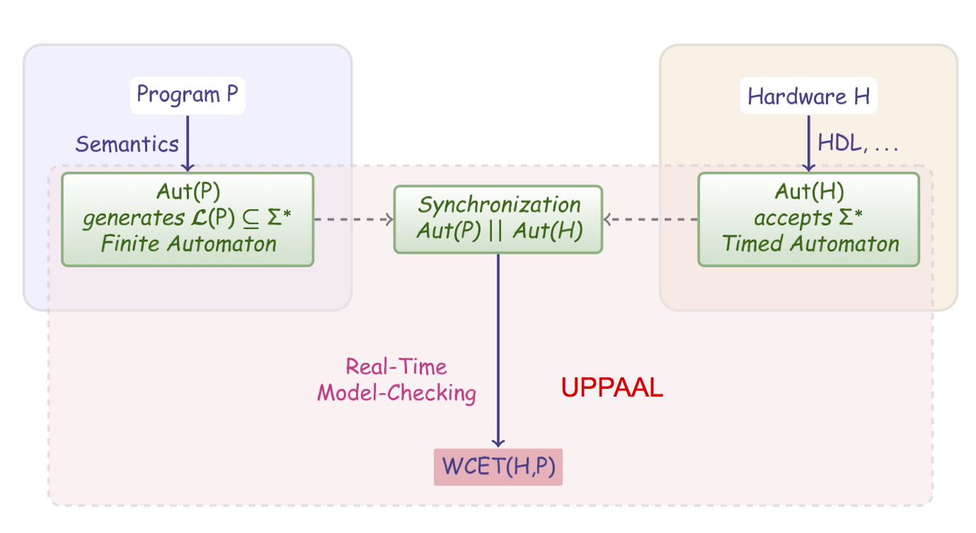
Our approach is summarised in the figure above.

Hardware, methodology

Tool Chain

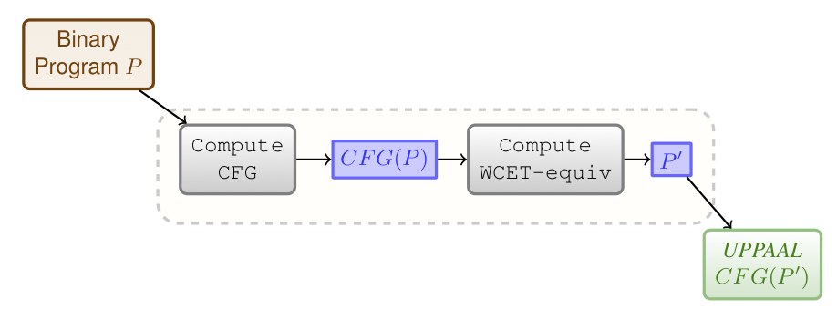Fig. 1: Tool Chain Overview

The architecture of our tool is given in Fig. 1.

The starting point is a binary program (that can be obtained with objdump using the CodeSourcery suite). This file is transformed into a Uppaal timed automaton by performing the following steps:

• generate the CFG of the program (Compute CFG)
• compute a reduced program (Compute WCET-equiv)
• generate the Uppaal description of the reduced program.

In the result file we embed models of the pipeline and the caches of the ARM920T. This produces a ready-to-analyse Uppaal file that generates the runs of the program on an ARM920T.

The WCET is computed by computing the largest value a clock (never reset in the program) can take in a final state. This amounts to checking a reachability property.

We have implemented the construction of the CFG (Compute CFG) and the computation of the WCET-equivalent program (Compute WCET-equiv). Together with a parser of ARM binary programs this makes a few thousand C++ lines of code. Our tool produces a bundle of files: a ready-to-analyse file containing the UPPAAL timed automata models of the program a binary P and the hardware models (the layout of the CFG is produced using dot), a dot file with the graph of the program and a ready-to-compile C++ file that contains a simulator of the program. This last file can be compiled and used to compute useful information like the ranges of registers. Notice that during the first phase ComputeCFG we compute the range of the stack pointer and thus the tool can also be used as a stack analyser.

Architecture of the ARM920T

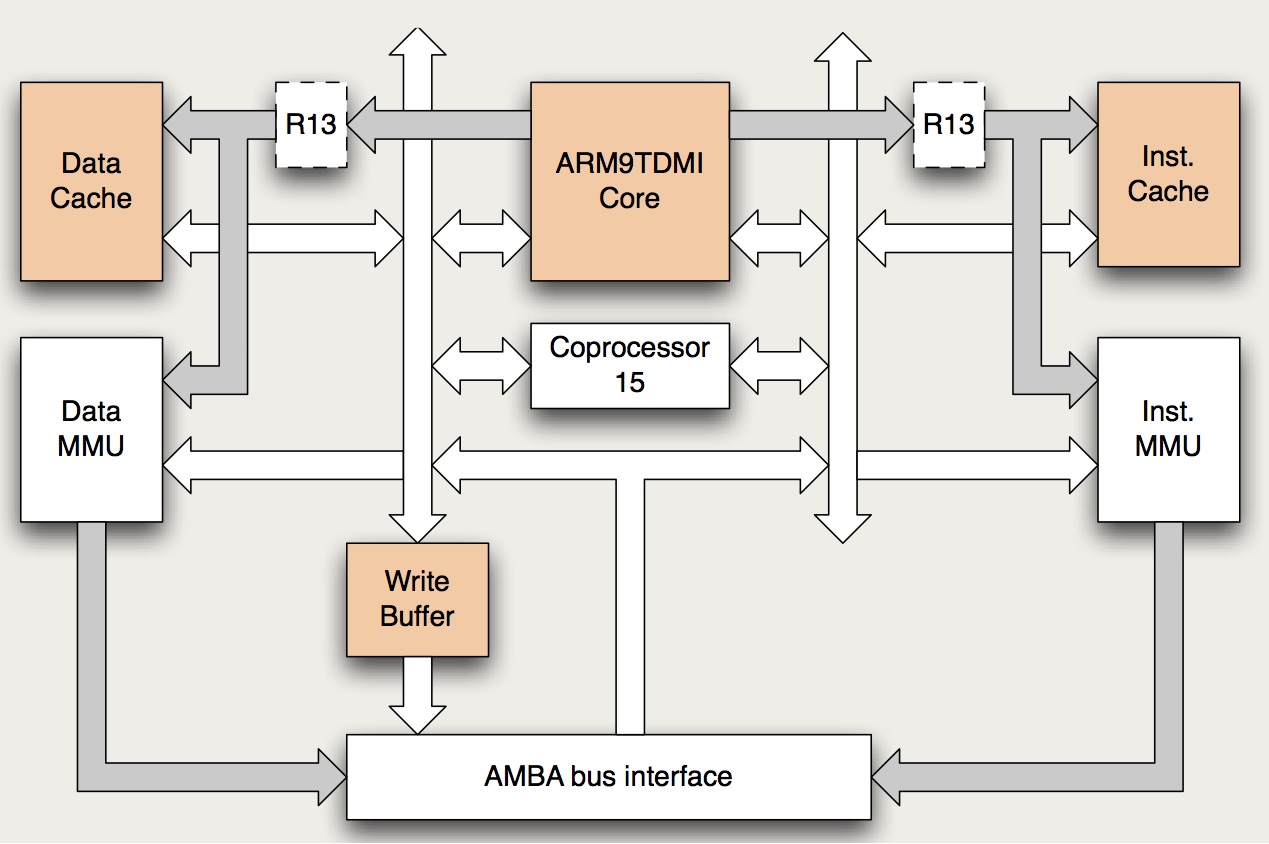Fig. 2: Simplified block diagram of the ARM920T.

The development board we model and use is an Armadeus APF9328 board which bears a 200MHz Freescale MC9328MXL micro-controller with an ARM920T processor. The processor embeds an ARM9TDMI core that implements the ARM v4T architecture. An overview of the architecture is given in Fig. 2. Gray arrows are address buses/connections. White arrows are data buses/connections. Both are 32 bits wide. Coprocessor 15 hosts control registers for the caches and the MMUs. Actually Register R13 (which should not be confused with the ARM9TDMI r13 register) is not duplicated and is located in Coprocessor 15. It hosts a process ID used for virtual address to physical address translation. Some blocks like the Write back Physical TAG RAM and various debug and/or coprocessor interfaces are not shown.

Methodology

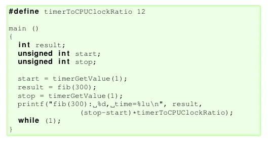Listing. 1: Wrapper program.

Original C sources files are available from the Mälardalen WCET Research Group. We provide the files (first column of Table 1) as we have slightly modified some of them: the WCET for most of the files is very small, and measurement errors are relatively large; this is why we have changed (when necessary and possible) the number of iterations in the C program. For example, the original C program for fib computes the Fibonacci number 30 and in our example we have computed fib(300) so that the WCET is larger and measurement errors are less than 1%. The program P to analyse is wrapped in a template function main: an example for program fib(300) is given in Listing 1.

Given P, we let t(P) be the wrapped program. Measuring the execution-time of P consists in (1) reading a hardware timer (timerGetValue) into a start variable, (2) calling the program P, and (3) reading the timer again in a stop variable and (4) printing¹ the difference stop − start. The function timerGetValue (assembly code) has been designed to read a hardware timer (See next paragraph). The measurement error is plus or minus 12 processor cycles. The program t(P) is compiled and linked. Running it on the ARM9 will print out the number of cycles taken by the program P: this figure is given in column “Measured WCET” in Table 1.

To faithfully compute the WCET of P using our method, we take as input of our tool chain t(P). t(P) is transformed (using Compute CFG and Slice) into a Uppaal automaton. In this automaton a dedicated clock GBL_CLK is reset when the instruction² of t(P) that reads the hardware timer flows out of the M stage (reading the timer in function timerGetValue is done using a load instruction). The final state of the automaton is reached when the second occurrence of the instruction that reads the timer flows out of the W stage. The computed WCET is given in column “Computed WCET” in Table 1. Column “Uppaal” in Table 1 gives the time Uppaal takes to check the property sup {WriteBackStage.DONE} : GBL\_CLK clock that gives the maximal value of a clock in a designated set of states. To do this we used a soon-to-be-released version of UPPAAL (64-bit, Academic UPPAAL 4.1.12 (rev. 5150), November 2012). With older versions of UPPAAL, files with large arrays take a very long time to parse due to some non-optimized library code and the verification times were badly impacted by this phase.

UPPAAL models and other files

UPPAAL models for the programs in Table  1 are available here. The archive contains the models and instructions how to compute the WCET with UPPAAL (verifyta). Another archive sources contains the C source, compiled ARM binary and the CFG for each analysed program: the .arm file is the assembly code we analyse and is obtained using objdump on the compiled C source, the .dot file gives some graphical representation of the CFG of the program (you should install GraphViz) to display it.

Results

Results in Table  1 are obtained with the latest hardware models and UPPAAL (64-bit, Academic UPPAAL 4.1.12 (rev. 5150), November 2012).

Comments on the Results

For the Single-Path programs the results show that our hardware formal model (and sliced program) contain enough details to capture the caches and pipeline features.

The second section Single-Path with MUL/SMULL requires some more explainations: when we compute the WCET using the UPPAAL models, we use an interval for durations of the instructions MUL/MLA and SMULL. Indeed the time it takes to perform one of this instruction depends on the data in the operands. For MUL/MLA the execution-time in the execution stage of the pipeline is within [3,6] cycles and for SMULL within [4,7].

The computed WCET is thus interval. Notice that there is no need for assuming that no timing anomalies occur as we do not assume that the duration of MUL/MLA or SMULL is the upper bound of the interval. The exploration of the state-space encompasses all the cases for all the possible durations of MUL/MLA and SMULL within their respective intervals. For the matmult program, we have measured the execution-time for two different input data: these data were intended to yield respectively the shortest and largest execution-time. Of course, we cannot guarantee that they actually yield the WCET. For instance for the O2 version, the binary program is optimized and it is rather difficult to guess which input data produces the WCET.

The last section Multiple-Path programs contains results for programs with data dependent decisions during the course of execution. The computed WCET takes into account all the possible choices. For measurements, we have again tried to choose the input that produces the WCET (for some of the programs this is difficult to claim that this choice is correct).

Overall, the results are very tight even on large execution-times (matmult-O0).

Model-Checking Binary Programs

The UPPAAL models we provide can also be used for model-checking functional (non quantitative) properties as well. It suffices to synchronize the prog template with a simple loop automaton that accepts/generates the fetch action. The examples zip files below contains this loop automaton (alwaysFetch) together with some properties that can be checked. It is for instance possible to check that the range of accessed memory cells is within a particular set, or to compute the max size of the stack, check for deadcode, etc. In the example file below, we compute the shortest path and longest path in the program insertsort-O2 using a clock: two steps of the program are separated by one time unit, hence the sup and inf values of the clock gives the longest and shortest paths in the program. We can also check that "loops" (or nodes that look like loop boundaries) can be iterated more than M times and hence compute loop bounds which is required for some tools to compute WCET. To compute loop bounds we can do a binary search and check the property A[] N ≤ K where N is a counter that is incremented every time a "loop" node is entered and K the expected bound. Notice that our computation of WCET does not rely on these loop bounds as the slice and variables needed to keep track of the control flow are included (and discovered) in the slicing phase.

The UPPAAL models of some programs we used for model checking properties are downloadable using the following link:

• bs-O0
• insertsort-O2

We provided a few examples to illustrate how we can model-check binary programs with UPPAAL but adding the alwaysFetch automaton to each file of Table 1 is straighforward and the method is applicable to the entire set of benchmarks of this table.

Statistical Model-Checking

The UPPAAL models obtained after the slicing phase can also be used to simulate traces of a binary program. This is a very nice feature as it is possible to use the statistical model-checking (see related references for details) approach to obtain more insights into the distribution of the execution times. It is also a good alternative to the computation of the WCET using the exhaustive approach in case it is impractical. In the sequel we give the transformed models of some programs of Table~1 that are ready for statistical model-checking. They slightly differ from the models of Table~1 as priorities and one-to-one communication can not be used in the current version of UPPAAL statistical model-checking. We have transformed the models of Table~1 obtained after slicing into models that use only 1) broadcast channels and 2) no priority. This way we can use the statistical model-checking feature in UPPAAL to obtain the probability distribution of the execution times.

The methodology we have used is the following:

• determine in the CFG the nodes at which non-determinitic choices can occur due to unknown inout data;
• assign a weight to each choice: the probability of firing an edge from the node is then the weight of the edge divided by the summation of the weights of the outgoing edges.

Notice that there are no probabilities on timing (as the system is time deterministic once a path is taken).

The NS example

Plot 1: ns-O0 distribution of execution times for p=1.

The ns-Ox (x=0,1,2) programs all look for a particular value in a MAX_NUM=5*5*5*5 matrix. When the value is found, the program terminates. We have added weights to the edges (in the binary program) where termination can happen as these are the only non-determistic choices in the program.

For example in ns-O0, there is only one such edge, 0x3350 (#13136). We want to encode the following facts regarding the input data for ns-O0:

• the key searched for is in the matrix with probabalility p in [0,1]
• when the key is in the matrix, the probability of finding it after looking up n elements is p/n.

We can encode this using the UPPAAL weights by making them dependent on the number elements already looked up in the matrix. The distribution of the execution times for ns-O0 with p=1 i.e.the key is always found (with default statistical parameters values in UPPAAL) is given by Plot 1.

For this program, according to Table 1 above, the (computed) WCET is 30968. The statistical property checked with UPPAAL is Pr[GBL_CLK<=35000](<> TheProg.DONE) where TheProg.DONE is true only when the last instruction of the program flows out of the last stage of the pipeline.

Plot 2: ns-O0 distribution of execution times for p=4/5.

Now if we set p=4/5 (key is found with probability 4/5) the distribution of execution times is given by Plot 2:

Accordingly the distribution shows that 1/5 of the 732 simulated runs actually have a duration close to the WCET (as the key is not found and all elements in the matrix are scanned) and the remaining runs durations (whent the key is found) are evenly distributed from the BCET to the WCET. We used UPPAAL 4.1.11 (rev5085) on a MacBook Air 11". 732 runs are simulated and the distribution of execution times is (as expected) evenly distributed from the BCET to the WCET.

Plot 3: ns-O1 distribution of execution times for p=1.

In Plot 3, we ran UPPAAL with the probability to find the key set to one and different settings for statistical parameters: width of buckets, probability of false negatives/positives in order to get a higher confidence level. Basically the blue bars chunk the x-axis into buckets of width 500 and the other bars (red and green) have width 200. As can be seen the distribution of the execution times is rather even.

To reproduce the results, open UPPAAL 4.1.11 and open one of the example files listed below. This should load the NTA model together with the properties to check. Check the property that looks like Pr[GBL_CLK<=Something](<> TheProg.DONE)). When it terminates, open the Plot Composer (Tool Tab) to display the simulation results. It is possible to play with this probability p to see the impact on the distribution of the execution times: it is defined as a constant in the template prog inthe UPPAAL models.

The Insertsort example

Plot 4: insertsort-O2 distribution of execution times.

The insertsort performs a insert sort. After each insertion, the list looks like (e1,e2,...ek,l,l1,l2,...lj) where (e1,e2,ek) is sorted and (l,l1,l2,lj) has to be inserted in the sorted list. In the version compiled with option -O2 we have added (dynamic) weights to the two non-deterministic choices in the program: 1) when a new element l to insert is compared with the maximum ek of the sorted sub-list and 2) when the new element l to insert is compared with other elements ek-1, ... e2, e1 of the sorted sub-list. We can then encode properties on the input data like: the input data (a list) is almost sorted by setting the propability that the element l to insert is larger than or equal ei to k-i. Results with different assumptions on the input data are given in Plot~4.

Plot 5: insertsort-O2 distribution of program steps (green)
and execution times (red).

It is also easy to obtain a comparison between the shape of the distribution of program steps and program execution times.

We can compute the probability Pr[#<=Something](<> TheProg.DONE)) on the NTA model using the alwaysFetch template and display the plot. The result is given on Plot 5. As can be seen on Plot 5, the distribution of the program steps and program execution times have the same shape.

The Binary Search example

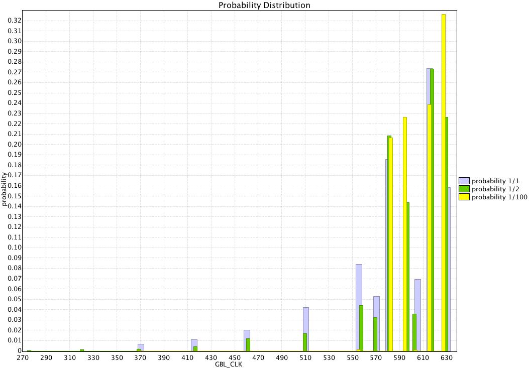Plot 6: bs800-O2 distribution of execution times
wrt probability of finding the key.

The binary sort analysis using statistical model-checking is given in Plot 6. We set probability to find the key in the set of 800 ordered values and annotate the UPPAAL models to reflect this. If the property to find the key in the set of 800 values is p=a/b, then a good approximtion for the weights of the UPPAAL transitions to find the key at iteration k in the binary search is a and not to find the key is 800/(2^k)*b-a. Plot 6 shows the statistics for the a/b=1/1,1/2 and 1/100.

ZIP Files and Other Examples

The UPPAAL models of the programs we used for the statistical model checking computation are downloadable using the following links:

• ns-O0
• ns-O1
• insertsort-O2
• bs-O2

To reproduce the results, open UPPAAL 4.1.11 and open one of the example files. This should load the NTA model together with the properties to check. Check the property that looks like Pr[GBL_CLK<=Something](<> TheProg.DONE)). When it terminates, open the Plot Composer (Tool Tab) to display the simulation results.

References

Our publications

Other Related publications